Attributes of numpy array
The important attributes of an array are:
- Dimension (
ndarray.ndim) - Shape (
ndarray.shape) - Size (
ndarray.size) - Data Type (
ndarray.dtype) - Item size (
ndarray.itemsize)
Let’s see the information that each of these properties provide
#import packages
import numpy as np
#create array
a = np.arange(20).reshape(4,5)
a
array([[ 0,  1,  2,  3,  4],
       [ 5,  6,  7,  8,  9],
       [10, 11, 12, 13, 14],
       [15, 16, 17, 18, 19]])
#Find the dimension
a.ndim
2
#Find the shape
a.shape
(4, 5)
#find the size
a.size
20
#find the data type
a.dtype
dtype('int64')
Creating array from list
#create a list
a_list = [[1, 2, 3, 4 ], [5, 6, 7, 8]]
print(type(a_list))

#create array from list

a_arr = np.array(a_list)
type(a_arr)
<class 'list'>
numpy.ndarray
Create arrays of known dimension, shape and size with initial placeholder values
b_arr = np.zeros((3,3,3))
b_arr
array([[[0., 0., 0.],
        [0., 0., 0.],
        [0., 0., 0.]],

       [[0., 0., 0.],
        [0., 0., 0.],
        [0., 0., 0.]],

       [[0., 0., 0.],
        [0., 0., 0.],
        [0., 0., 0.]]])
c_arr = np.ones((3,3,3))
c_arr
array([[[1., 1., 1.],
        [1., 1., 1.],
        [1., 1., 1.]],

       [[1., 1., 1.],
        [1., 1., 1.],
        [1., 1., 1.]],

       [[1., 1., 1.],
        [1., 1., 1.],
        [1., 1., 1.]]])
Create Sequence of numbers
Numpy provides arange function. This works similar to python built-in range function.
d_arr = np.arange(10, 110, 5) #start at 10, stop at 110, step 5
d_arr
array([ 10,  15,  20,  25,  30,  35,  40,  45,  50,  55,  60,  65,  70,
        75,  80,  85,  90,  95, 100, 105])
If we are more interested in the number of elements to return instead of the interval to use, we use linspace
e_arr = np.linspace(0, 40, 5) #Give 5 linearly spaced values starting at 10 and ending at 100.
e_arr
array([ 0., 10., 20., 30., 40.])
Basic Operation
Arithmetic operation are usually applied element-wise
a = np.arange(25, step=5)
b = np.linspace(2, 10, 5)
print(a)
print(b)
[ 0  5 10 15 20]
[ 2.  4.  6.  8. 10.]
#add the two arrays
a + b
array([ 2., 9., 16., 23., 30.])
#multiply the arrays
a*b
array([ 0., 20., 60., 120., 200.])
#Perform logical operation
a == 5
array([False, True, False, False, False])
Note that the * operation performs element wise operation unlike the usual matrix multiplication. The matrix multiplication can be achieved using @ or nparray.dot() method
a = np.array([[1, 3, 5],
                [2, 4, 6],
                [1,1,2]]) #3x3

b = np.array([[2],
                [3],
                [4]]) #3x1
We created two matrices a and b above. a is 3 x 3 and b is 3 x 1. The intention is to find the matrix mulplication so our result so be a 3 x 1 matrix. Let’s see and compare the result of * operator, @ operator and dot function
# * operator
a*b
array([[ 2,  6, 10],
       [ 6, 12, 18],
       [ 4,  4,  8]])
# @ operator
a@b
array([[31],
       [40],
       [13]])
# dot function
a.dot(b)
array([[31],
       [40],
       [13]])
- operation performs element-wise operation which is not what we want. Both @ and dot function did the intended matrix multiplication. It is important to understand how numpy method operates on array element. Many unitary operations like sum(), max(), min(), mean() operates on numpy arrays as if they were list of values regardless of their shape. It is therefore important to specify the required axis of operation to achieve desired result.
# Find the sum of all elements
a = np.array([[1, 3, 5],
                [2, 4, 6],
                [1,1,2]])
a.sum()
25
The code above calculates the sum of all the elements in the array. Axis can be specified to change this behaviour to achieve desired result
#calculate sum along each column
a = np.array([[1, 3, 5],
                [2, 4, 6],
                [1,1,2]])
a.sum(axis=0)
array([ 4, 8, 13])
#calculate sum along different axis
b = np.array([[[1, 3, 5],
                [2, 4, 6],
                [1,1,2]],

                [[11, 13, 15],
                [12, 14, 16],
                [11,11,12]]])

b.sum(axis=0)
array([[12, 16, 20],
       [14, 18, 22],
       [12, 12, 14]])
b.sum(axis=1)
array([[ 4,  8, 13],
       [34, 38, 43]])
b.sum(axis = 2)
array([[ 9, 12,  4],
       [39, 42, 34]])
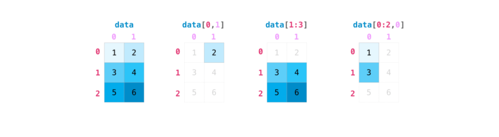
Indexing and Slicing
One dimensional numpy array can be indexed and sliced in a similar way as python list. Indexing is achieved by calling the appropriate element position.
For more than one dimensional array, use , to separate the axis. It is important to note that indexing in array and list starts with 0.
To slice between the elements, use a:b. The operation will slice from element at position a up to but not including position b.
#Indexing one-dimensional list  and array
a_list = [1, 2, 3, 4, 5]
a_arr = np.array(a_list)

#index first element of list and print
print('First elemet of the list:', a_list[0])

#index first element of array and print
print('First element of the array', a_arr[0])

# Slicing first two elements of list
print('First two elements of the list:', a_list[0:2])

# Slicing first two elements of array
print('First two elements of the array:', a_arr[0:2])

#Slice the last two elements of the list
print('Last two elements of the list:', a_list[-2:])

#Slice the last two elements of the array
print('Last two elements of the array:', a_arr[-2:])
First elemet of the list: 1
First element of the array 1
First two elements of the list: [1, 2]
First two elements of the array: [1 2]
Last two elements of the list: [4, 5]
Last two elements of the array: [4 5]
# Indexing and slicing two-dimensional array

b_arr = np.array([[1, 3, 5],
          [2, 4, 6],
          [1,1,2]])

# Index element in the first row and second column of the array
print('Element in the first row and second column:', b_arr[0,1])

#When fewer indices are provided, the missing indices are considered complete slices.
print('All elements of the third row of the array:', b_arr[2]) #equivalent to a_arr[2,:]

# last two rows and first two columns of the array
print('Last two rows and first two columns of the array:', b_arr[-2:,:2])
Element in the first row and second column: 3
All elements of the third row of the array: [1 1 2]
Last two rows and first two columns of the array: [[2 4]
 [1 1]]
Iterating over an array
Iterating one-dimensional array is similar to iterating a list: It goes over each element. Iterating more than one-dimensional array is done with respect to the first axis. To perform an operation on each element of the array, use flat attribute
# Iterate ove one-dimensional array
for i in a_arr:
    print(i)
1
2
3
4
5
# iterating over axis of a two-dimensional array
for i in b_arr:
    print(i)
[1 3 5]
[2 4 6]
[1 1 2]
#iterating over elements of a two-dimensional array
for i in b_arr.flat:
    print(i)
1
3
5
2
4
6
1
1
2