Exploratory data analysis with Python

Share This Post

This notebook is a practical demonstration of an exploratory data analysis task. For this task, we want to understand how completion rates differ for different types of students and different types of schools. We want to look at this by:

  • Student race
  • Admission policy and rate
  • Public/private status (the documentation describes this as “control” — what is the legal or financial control status of the school?)

    We will work with the data set underlying the Department of Education’s College Scorecard. This is a medium-sized data set. We will only work with the most recent cohort’s data.

Motivation.

The data was created to promote openness by giving students and families the ability to assess different colleges are preparing performing and preparing its students for the workforce. The public, particularly students and families can use the data to compare the costs and results of various universities.

The instituition data is part of the large College Scoredcard project of the U.S Department of Education. The data is collected annually through surveys administered by the Department of Education’s National Center for Education Statistics (NCES), IPEDS is the primary source of data on postsecondary education institutions in the United States.

Composition

There are about 10 instances in the data:

  1. Academics : This instance describes the types of academic offerings available at each institution.
  2. Admissions : This instance This information describes the admissions rate and SAT/ACT scores of students aids.
  3. Aid : This instance covers information on financial aid including Pell Grants and federal student loans which help many students particularly low-incone students access and afford a higher education.
  4. Completion : This instance contains information on college completion which determines other positive outcones such as finding a job and succesfully repaying student loans.
  5. Cost : This instance contains information about the costs to students of an institution which can provide important context for students and families as they seek to evaluate the tradeoffs of access, affordability, and outcomes.
  6. Earnings : This instance contains information on the earnings and employment prospects of former students.
  7. Repayment : This instance provides information on the debt burden of attending college and the loan performance metrics for each institution.
  8. School : This instance provides basic descriptive information about the institution in question. These include: identifiers, location, degree type and profile, programs offered, and the academic profile of students enrolled.
  9. Student : This instance identifies demographic and other details about the student body of the institution. The category under this include number of undergraduate students, student body by race, gender, age, Part-Time/Full-Time status, family income

Q4: Does the dataset identify any subpopulations (e.g., by age, gender)? If so, please describe how these subpopulations are identified and
provide a description of their respective distributions within the dataset.

Yes. The instituitional data contains several elements that identify demographic based on their age, sex and race. The race and gender are reported by the instituitions to IPEDS in the fall enrollment components and rely on student’s self-reported race and gender data as collected by the instituition.

In [ ]:
#import packages

import numpy as np
import pandas as pd
import matplotlib.pyplot as plt
import seaborn as sns

0. Data Cleaning

read the data

In [ ]:
# read the csv file

schools = pd.read_csv('../../Data/Most-Recent-Cohorts-Institution_04262022/Most-Recent-Cohorts-Institution.csv',
            usecols= ['INSTNM', 'CITY', 'STABBR', 'ST_FIPS', 'CONTROL', 'HIGHDEG', 'ICLEVEL', 'C150_4', 'C150_4_POOLED', 'C150_L4', 'C150_L4_POOLED', 'C100_4', 'C100_4_POOLED', 'C100_L4', 'C100_L4_POOLED',
            'OPENADMP', 'ADM_RATE', 'ADM_RATE_ALL'])

#create a dictionary variable to use for encoding ST_FIPS column
state_name = {1: 'Alabama', 2 : 'Alaska', 4 : 'Arizona', 5 : 'Arkansas', 6 : 'California', 8 : 'Colorado', 9 : 'Connecticut', 10 : 'Delaware', 
            11 : 'District of Columbia', 12 : 'Florida', 13 : 'Georgia', 15 : 'Hawaii', 16 : 'Idaho', 17 : 'Illinois', 18 : 'Indiana', 19 : 'Iowa', 20 : 'Kansas', 
            21: 'Kentucky', 22 : 'Louisiana', 23 : 'Maine', 24 : 'Maryland', 25 : 'Massachusetts', 26 : 'Michigan', 27 : 'Minnesota', 28 : 'Mississippi', 29 : 'Missouri', 30 : 'Montana',
            31 : 'Nebraska', 32 : 'Nevada', 33 : 'New Hampshire', 34 : 'New Jersey', 35 : 'New Mexico', 36 : 'New York', 37 : 'North Carolina', 38 : 'North Dakota', 39: 'Ohio', 40 : 'Oklahoma',
            41 : 'Oregon', 42 : 'Pennsylvania', 44 : 'Rhode Island', 45 : 'South Carolina', 46 : 'South Dakota', 47 : 'Tennessee', 48 : 'Texas', 49 : 'Utah', 50 : 'Vermont',
            51 : 'Virginia', 53 : 'Washington', 54 : 'West Virginia', 55 : 'Wisconsin', 56 : 'Wyoming', 60 : 'American Samoa', 64 : 'Federated States of Micronesia', 66 : 'Guam',
            69 : 'Northern Mariana Islands', 70 : 'Palau', 72 : 'Puerto Rico', 78 : 'Virgin Islands'}
# encode ST_FIPS to the state name and drop the column
schools['STATE'] = schools.ST_FIPS.map(state_name)
schools = schools.drop(['ST_FIPS'], axis = 1)

# create a dictionary variable to use for encoding CONTROL
control_name = {1 : 'Public', 2 : 'Private, Nonprofit', 3 : 'Proprietary'}
# encode CONTROL column and drop the column
schools['CONTROL_STATUS'] = schools.CONTROL.map(control_name)
schools = schools.drop(['CONTROL'], axis = 1)

# create a dictionary to use for encoding Highest award column
highdegree_name = {0 : 'Non-degree-granting', 1: 'Certificate degree', 2 : 'Associate degree', 3 : 'Bachelor degree' , 4 : 'Graduate degree'}
# encode HIGHDEG column and drop the column
schools['HIGHDEG_TYPE'] = schools.HIGHDEG.map(highdegree_name)
schools = schools.drop(['HIGHDEG'], axis = 1)

# create a dictionary to use for encoding Level of Instituition
iclevel_name = {1 : '4 Year', 2 : '2 Year', 3 : 'Less than 2 year'}
# encode ICLEVEL column and dropm the column
schools['ICLEVEL_TYPE'] = schools.ICLEVEL.map(iclevel_name)
schools = schools.drop(['ICLEVEL'], axis= 1) 

schools
Out[ ]:
INSTNM CITY STABBR ADM_RATE ADM_RATE_ALL C150_4 C150_L4 C150_4_POOLED C150_L4_POOLED C100_4 C100_L4 OPENADMP C100_4_POOLED C100_L4_POOLED STATE CONTROL_STATUS HIGHDEG_TYPE ICLEVEL_TYPE
0 Alabama A & M University Normal AL 0.8965 0.8965 0.2866 NaN 0.2918 NaN 0.1052 NaN 2.0 0.0929 NaN Alabama Public Graduate degree 4 Year
1 University of Alabama at Birmingham Birmingham AL 0.8060 0.8060 0.6117 NaN 0.6229 NaN 0.3816 NaN 2.0 0.3920 NaN Alabama Public Graduate degree 4 Year
2 Amridge University Montgomery AL NaN NaN 0.2500 NaN 0.2857 NaN 0.2500 NaN 1.0 0.2400 NaN Alabama Private, Nonprofit Graduate degree 4 Year
3 University of Alabama in Huntsville Huntsville AL 0.7711 0.7711 0.5714 NaN 0.5740 NaN 0.3109 NaN 2.0 0.2914 NaN Alabama Public Graduate degree 4 Year
4 Alabama State University Montgomery AL 0.9888 0.9888 0.3177 NaN 0.3235 NaN 0.1462 NaN 2.0 0.1571 NaN Alabama Public Graduate degree 4 Year
6657 Pennsylvania State University-Penn State Wilke… Lehman PA NaN 0.7827 NaN NaN NaN NaN NaN NaN NaN NaN NaN Pennsylvania Public Non-degree-granting 4 Year
6658 Pennsylvania State University-Penn State York York PA NaN 0.7827 NaN NaN NaN NaN NaN NaN NaN NaN NaN Pennsylvania Public Non-degree-granting 4 Year
6659 Pennsylvania State University-Penn State Great… Malvern PA NaN 0.7827 NaN NaN NaN NaN NaN NaN NaN NaN NaN Pennsylvania Public Non-degree-granting 4 Year
6660 Pennsylvania State University-Penn State Harri… Middletown PA NaN 0.7827 NaN NaN NaN NaN NaN NaN NaN NaN NaN Pennsylvania Public Non-degree-granting 4 Year
6661 Pennsylvania State University-Penn State Brand… Media PA NaN 0.7827 NaN NaN NaN NaN NaN NaN NaN NaN NaN Pennsylvania Public Non-degree-granting 4 Year

6662 rows × 18 columns

In [ ]:
# check the data structure
schools.info()
<class 'pandas.core.frame.DataFrame'>
RangeIndex: 6662 entries, 0 to 6661
Data columns (total 18 columns):
 #   Column          Non-Null Count  Dtype  
---  ------          --------------  -----  
 0   INSTNM          6662 non-null   object 
 1   CITY            6662 non-null   object 
 2   STABBR          6662 non-null   object 
 3   ADM_RATE        1960 non-null   float64
 4   ADM_RATE_ALL    2234 non-null   float64
 5   C150_4          2270 non-null   float64
 6   C150_L4         3180 non-null   float64
 7   C150_4_POOLED   2292 non-null   float64
 8   C150_L4_POOLED  3207 non-null   float64
 9   C100_4          2007 non-null   float64
 10  C100_L4         3180 non-null   float64
 11  OPENADMP        5691 non-null   float64
 12  C100_4_POOLED   2046 non-null   float64
 13  C100_L4_POOLED  3207 non-null   float64
 14  STATE           6661 non-null   object 
 15  CONTROL_STATUS  6662 non-null   object 
 16  HIGHDEG_TYPE    6662 non-null   object 
 17  ICLEVEL_TYPE    6662 non-null   object 
dtypes: float64(11), object(7)
memory usage: 937.0+ KB

Fill in the missing values

There are lot of missing values in the completion rate columns as shown by the info above. There are about 6662 records of instuitions in the database but the completion rate variables have way less. For example, C150_4 has 2270 non-null values while C150_L4 has about 3180. A way to fill the missing values is to combine these columns if there are no schools in both categories.

In [ ]:
#find out if there is any school in both 4 years and less than 4 years column
print(len(schools[schools['C100_4'] == schools['C100_L4']]))
print(len(schools[schools['C150_4'] == schools['C150_L4']]))
0
0
In [ ]:
#Filling the 4 years column with less than 4 years column
schools['C_100'] = schools['C100_4'].combine_first(schools['C100_L4'])
schools['C_100_POOLED'] = schools['C100_4_POOLED'].combine_first(schools['C100_L4_POOLED'])
schools['C_150'] =  schools['C150_4'].combine_first(schools['C150_L4'])
schools['C_150_POOLED'] = schools['C150_4_POOLED'].combine_first(schools['C150_L4_POOLED'])

#drop the other completion rate columns after filling
schools = schools.drop(['C100_4', 'C100_L4', 'C100_4_POOLED', 'C100_L4_POOLED', 'C150_4', 'C150_L4', 'C150_4_POOLED', 'C150_L4_POOLED'], axis = 1)

schools.info()
<class 'pandas.core.frame.DataFrame'>
RangeIndex: 6662 entries, 0 to 6661
Data columns (total 14 columns):
 #   Column          Non-Null Count  Dtype  
---  ------          --------------  -----  
 0   INSTNM          6662 non-null   object 
 1   CITY            6662 non-null   object 
 2   STABBR          6662 non-null   object 
 3   ADM_RATE        1960 non-null   float64
 4   ADM_RATE_ALL    2234 non-null   float64
 5   OPENADMP        5691 non-null   float64
 6   STATE           6661 non-null   object 
 7   CONTROL_STATUS  6662 non-null   object 
 8   HIGHDEG_TYPE    6662 non-null   object 
 9   ICLEVEL_TYPE    6662 non-null   object 
 10  C_100           5187 non-null   float64
 11  C_100_POOLED    5253 non-null   float64
 12  C_150           5450 non-null   float64
 13  C_150_POOLED    5499 non-null   float64
dtypes: float64(7), object(7)
memory usage: 728.8+ KB

Selecting Variables

The completion rates for full-time, first-time students who complete within 100 or 150 percent of the expected time to completion are represented by C_100 and C_150 variables respectively. However, only the 150 percent rates are available disaggregated by race. So C_150 would make the most of sense in the context of this task. C_100_POOLED and C_150_POOLED variables are pooled completion rates across two years rolling basis. For self-consistent analysis, I use the normal completion rate variables and not the pooled varaibles.

In [ ]:
#drop the POOLED completion rates

schools = schools.drop(['C_100_POOLED', 'C_150_POOLED'], axis = 1)

schools.info()
<class 'pandas.core.frame.DataFrame'>
RangeIndex: 6662 entries, 0 to 6661
Data columns (total 12 columns):
 #   Column          Non-Null Count  Dtype  
---  ------          --------------  -----  
 0   INSTNM          6662 non-null   object 
 1   CITY            6662 non-null   object 
 2   STABBR          6662 non-null   object 
 3   ADM_RATE        1960 non-null   float64
 4   ADM_RATE_ALL    2234 non-null   float64
 5   OPENADMP        5691 non-null   float64
 6   STATE           6661 non-null   object 
 7   CONTROL_STATUS  6662 non-null   object 
 8   HIGHDEG_TYPE    6662 non-null   object 
 9   ICLEVEL_TYPE    6662 non-null   object 
 10  C_100           5187 non-null   float64
 11  C_150           5450 non-null   float64
dtypes: float64(5), object(7)
memory usage: 624.7+ KB

ADMISSIONS

There are two variables that describe the admissions practices. OPENADMP indicates whether it has an open admissions policy. 1 -Yes, 2 – No, 3 – Does not enrol first-time student. Second, schools that do not have an open admissions policy (2) report the admission rate. For institutions with multiple branches,
ADM_RATE includes the admissions rate at each campus, while ADM_RATE_ALL represents the admissions rate across all campuses.

We’re going to bucketize the admissions policy. I defined three categories of schools:

  • Open-admission schools
  • Low-selectivity schools, where the admission rate is higher than the median admission rate
  • High-selectivity schools, where the admission rate is lower than the median admission rate
In [ ]:
# calculate the median admission rate for ADM_RATE and ADM_RATE_ALL
adm_median = schools['ADM_RATE'].median()
adm_median_all = schools['ADM_RATE_ALL'].median()

print(adm_median)
print(adm_median_all)
0.7518
0.7596499999999999
In [ ]:
#Convert admission rate to categorical values

# Bucketize the ADM_RATE variable
schools['ADM'] = 'Open-admission'
schools.loc[schools['ADM_RATE'] < adm_median, 'ADM'] = 'High-selectivity'
schools.loc[schools['ADM_RATE'] > adm_median, 'ADM'] = 'Low-selectivity'

#Bucketize the ADM_RATE_ALL variable
schools['ADM_ALL'] = 'Open-admission'
schools.loc[schools['ADM_RATE_ALL'] < adm_median_all, 'ADM_ALL'] = 'High-selectivity'
schools.loc[schools['ADM_RATE_ALL'] > adm_median_all, 'ADM_ALL'] = 'Low-selectivity'

schools
Out[ ]:
INSTNM CITY STABBR ADM_RATE ADM_RATE_ALL OPENADMP STATE CONTROL_STATUS HIGHDEG_TYPE ICLEVEL_TYPE C_100 C_150 ADM ADM_ALL
0 Alabama A & M University Normal AL 0.8965 0.8965 2.0 Alabama Public Graduate degree 4 Year 0.1052 0.2866 Low-selectivity Low-selectivity
1 University of Alabama at Birmingham Birmingham AL 0.8060 0.8060 2.0 Alabama Public Graduate degree 4 Year 0.3816 0.6117 Low-selectivity Low-selectivity
2 Amridge University Montgomery AL NaN NaN 1.0 Alabama Private, Nonprofit Graduate degree 4 Year 0.2500 0.2500 Open-admission Open-admission
3 University of Alabama in Huntsville Huntsville AL 0.7711 0.7711 2.0 Alabama Public Graduate degree 4 Year 0.3109 0.5714 Low-selectivity Low-selectivity
4 Alabama State University Montgomery AL 0.9888 0.9888 2.0 Alabama Public Graduate degree 4 Year 0.1462 0.3177 Low-selectivity Low-selectivity
6657 Pennsylvania State University-Penn State Wilke… Lehman PA NaN 0.7827 NaN Pennsylvania Public Non-degree-granting 4 Year NaN NaN Open-admission Low-selectivity
6658 Pennsylvania State University-Penn State York York PA NaN 0.7827 NaN Pennsylvania Public Non-degree-granting 4 Year NaN NaN Open-admission Low-selectivity
6659 Pennsylvania State University-Penn State Great… Malvern PA NaN 0.7827 NaN Pennsylvania Public Non-degree-granting 4 Year NaN NaN Open-admission Low-selectivity
6660 Pennsylvania State University-Penn State Harri… Middletown PA NaN 0.7827 NaN Pennsylvania Public Non-degree-granting 4 Year NaN NaN Open-admission Low-selectivity
6661 Pennsylvania State University-Penn State Brand… Media PA NaN 0.7827 NaN Pennsylvania Public Non-degree-granting 4 Year NaN NaN Open-admission Low-selectivity

6662 rows × 14 columns

TASK REQUIREMENT

1. A basic structural description of the data set:

  • How many schools and variables?
  • How many schools are there per state?
  • How are schools-per-state distributed? Compute a state-level variable ‘# of schools’, and describe its distribution numerically and visually.
In [ ]:
schools
Out[ ]:
INSTNM CITY STABBR ADM_RATE ADM_RATE_ALL OPENADMP STATE CONTROL_STATUS HIGHDEG_TYPE ICLEVEL_TYPE C_100 C_150 ADM ADM_ALL
0 Alabama A & M University Normal AL 0.8965 0.8965 2.0 Alabama Public Graduate degree 4 Year 0.1052 0.2866 Low-selectivity Low-selectivity
1 University of Alabama at Birmingham Birmingham AL 0.8060 0.8060 2.0 Alabama Public Graduate degree 4 Year 0.3816 0.6117 Low-selectivity Low-selectivity
2 Amridge University Montgomery AL NaN NaN 1.0 Alabama Private, Nonprofit Graduate degree 4 Year 0.2500 0.2500 Open-admission Open-admission
3 University of Alabama in Huntsville Huntsville AL 0.7711 0.7711 2.0 Alabama Public Graduate degree 4 Year 0.3109 0.5714 Low-selectivity Low-selectivity
4 Alabama State University Montgomery AL 0.9888 0.9888 2.0 Alabama Public Graduate degree 4 Year 0.1462 0.3177 Low-selectivity Low-selectivity
6657 Pennsylvania State University-Penn State Wilke… Lehman PA NaN 0.7827 NaN Pennsylvania Public Non-degree-granting 4 Year NaN NaN Open-admission Low-selectivity
6658 Pennsylvania State University-Penn State York York PA NaN 0.7827 NaN Pennsylvania Public Non-degree-granting 4 Year NaN NaN Open-admission Low-selectivity
6659 Pennsylvania State University-Penn State Great… Malvern PA NaN 0.7827 NaN Pennsylvania Public Non-degree-granting 4 Year NaN NaN Open-admission Low-selectivity
6660 Pennsylvania State University-Penn State Harri… Middletown PA NaN 0.7827 NaN Pennsylvania Public Non-degree-granting 4 Year NaN NaN Open-admission Low-selectivity
6661 Pennsylvania State University-Penn State Brand… Media PA NaN 0.7827 NaN Pennsylvania Public Non-degree-granting 4 Year NaN NaN Open-admission Low-selectivity

6662 rows × 14 columns

In [ ]:
schools['INSTNM'].nunique()
Out[ ]:
6530

There are about 6530 schools

In [ ]:
schools.groupby('STATE')['INSTNM'].count()
Out[ ]:
STATE
Alabama                            87
Alaska                              9
American Samoa                      1
Arizona                           120
Arkansas                           90
California                        705
Colorado                           94
Connecticut                        78
Delaware                           19
District of Columbia               26
Federated States of Micronesia      1
Florida                           394
Georgia                           174
Guam                                3
Hawaii                             23
Idaho                              39
Illinois                          253
Indiana                           136
Iowa                               77
Kansas                             79
Kentucky                           89
Louisiana                         121
Maine                              37
Maryland                           84
Massachusetts                     153
Michigan                          187
Minnesota                         112
Mississippi                        59
Missouri                          157
Montana                            32
Nebraska                           40
Nevada                             37
New Hampshire                      36
New Jersey                        165
New Mexico                         46
New York                          450
North Carolina                    178
North Dakota                       27
Northern Mariana Islands            1
Ohio                              288
Oklahoma                          104
Oregon                             76
Palau                               1
Pennsylvania                      345
Puerto Rico                       156
Rhode Island                       23
South Carolina                     98
South Dakota                       27
Tennessee                         157
Texas                             429
Utah                               68
Vermont                            20
Virgin Islands                      2
Virginia                          167
Washington                        105
West Virginia                      72
Wisconsin                          94
Wyoming                            10
Name: INSTNM, dtype: int64

The dataframe above shows the number of schools per state.

In [ ]:
num_schools = schools.groupby('STATE')['INSTNM'].count()

# convert the series to dataframe
num_schools = num_schools.to_frame().reset_index()
#rename the column
num_schools = num_schools.rename(columns={"INSTNM": "COUNT"})
num_schools
Out[ ]:
STATE COUNT
0 Alabama 87
1 Alaska 9
2 American Samoa 1
3 Arizona 120
4 Arkansas 90
5 California 705
6 Colorado 94
7 Connecticut 78
8 Delaware 19
9 District of Columbia 26
10 Federated States of Micronesia 1
11 Florida 394
12 Georgia 174
13 Guam 3
14 Hawaii 23
15 Idaho 39
16 Illinois 253
17 Indiana 136
18 Iowa 77
19 Kansas 79
20 Kentucky 89
21 Louisiana 121
22 Maine 37
23 Maryland 84
24 Massachusetts 153
25 Michigan 187
26 Minnesota 112
27 Mississippi 59
28 Missouri 157
29 Montana 32
30 Nebraska 40
31 Nevada 37
32 New Hampshire 36
33 New Jersey 165
34 New Mexico 46
35 New York 450
36 North Carolina 178
37 North Dakota 27
38 Northern Mariana Islands 1
39 Ohio 288
40 Oklahoma 104
41 Oregon 76
42 Palau 1
43 Pennsylvania 345
44 Puerto Rico 156
45 Rhode Island 23
46 South Carolina 98
47 South Dakota 27
48 Tennessee 157
49 Texas 429
50 Utah 68
51 Vermont 20
52 Virgin Islands 2
53 Virginia 167
54 Washington 105
55 West Virginia 72
56 Wisconsin 94
57 Wyoming 10
In [ ]:
num_schools.describe()
Out[ ]:
COUNT
count 58.000000
mean 114.844828
std 131.155031
min 1.000000
25% 28.250000
50% 81.500000
75% 155.250000
max 705.000000
In [ ]:
num_schools.plot.bar(x = 'STATE', y = 'COUNT', figsize=(18,10))
Out[ ]:
<AxesSubplot:xlabel='STATE'>

There is median of 81 schools in the states. Atleast one school in each state. California has the highest number of schools (705).

2. The distribution of the overall completion rate:

  • Provide choice of completion rate variable with a justification for that choice.
  • Describe the distribution of that variable numerically and visually.
  • What is the mean? Is the distribution skewed?

I selected C_100 and C_150 as the completion rates. The rational for this has been explained in the selection of variable section above.

In [ ]:
schools
Out[ ]:
INSTNM CITY STABBR ADM_RATE ADM_RATE_ALL OPENADMP STATE CONTROL_STATUS HIGHDEG_TYPE ICLEVEL_TYPE C_100 C_150 ADM ADM_ALL
0 Alabama A & M University Normal AL 0.8965 0.8965 2.0 Alabama Public Graduate degree 4 Year 0.1052 0.2866 Low-selectivity Low-selectivity
1 University of Alabama at Birmingham Birmingham AL 0.8060 0.8060 2.0 Alabama Public Graduate degree 4 Year 0.3816 0.6117 Low-selectivity Low-selectivity
2 Amridge University Montgomery AL NaN NaN 1.0 Alabama Private, Nonprofit Graduate degree 4 Year 0.2500 0.2500 Open-admission Open-admission
3 University of Alabama in Huntsville Huntsville AL 0.7711 0.7711 2.0 Alabama Public Graduate degree 4 Year 0.3109 0.5714 Low-selectivity Low-selectivity
4 Alabama State University Montgomery AL 0.9888 0.9888 2.0 Alabama Public Graduate degree 4 Year 0.1462 0.3177 Low-selectivity Low-selectivity
6657 Pennsylvania State University-Penn State Wilke… Lehman PA NaN 0.7827 NaN Pennsylvania Public Non-degree-granting 4 Year NaN NaN Open-admission Low-selectivity
6658 Pennsylvania State University-Penn State York York PA NaN 0.7827 NaN Pennsylvania Public Non-degree-granting 4 Year NaN NaN Open-admission Low-selectivity
6659 Pennsylvania State University-Penn State Great… Malvern PA NaN 0.7827 NaN Pennsylvania Public Non-degree-granting 4 Year NaN NaN Open-admission Low-selectivity
6660 Pennsylvania State University-Penn State Harri… Middletown PA NaN 0.7827 NaN Pennsylvania Public Non-degree-granting 4 Year NaN NaN Open-admission Low-selectivity
6661 Pennsylvania State University-Penn State Brand… Media PA NaN 0.7827 NaN Pennsylvania Public Non-degree-granting 4 Year NaN NaN Open-admission Low-selectivity

6662 rows × 14 columns

In [ ]:
com = schools[['C_100', 'C_150']]
com
Out[ ]:
C_100 C_150
0 0.1052 0.2866
1 0.3816 0.6117
2 0.2500 0.2500
3 0.3109 0.5714
4 0.1462 0.3177
6657 NaN NaN
6658 NaN NaN
6659 NaN NaN
6660 NaN NaN
6661 NaN NaN

6662 rows × 2 columns

In [ ]:
com.describe()
Out[ ]:
C_100 C_150
count 5187.000000 5450.000000
mean 0.373388 0.557012
std 0.270354 0.233730
min 0.000000 0.000000
25% 0.148400 0.371500
50% 0.328100 0.574500
75% 0.567700 0.733300
max 1.000000 1.000000
In [ ]:
plt.hist(com['C_100'], bins = 20)
Out[ ]:
(array([575., 330., 405., 375., 360., 376., 327., 272., 258., 249., 273.,
        232., 188., 190., 163., 162., 136., 112.,  79., 125.]),
 array([0.  , 0.05, 0.1 , 0.15, 0.2 , 0.25, 0.3 , 0.35, 0.4 , 0.45, 0.5 ,
        0.55, 0.6 , 0.65, 0.7 , 0.75, 0.8 , 0.85, 0.9 , 0.95, 1.  ]),
 <BarContainer object of 20 artists>)
In [ ]:
plt.hist(com['C_150'], bins = 20)
Out[ ]:
(array([ 69.,  39.,  85., 171., 236., 299., 331., 286., 312., 297., 419.,
        391., 410., 432., 438., 340., 301., 213., 178., 203.]),
 array([0.  , 0.05, 0.1 , 0.15, 0.2 , 0.25, 0.3 , 0.35, 0.4 , 0.45, 0.5 ,
        0.55, 0.6 , 0.65, 0.7 , 0.75, 0.8 , 0.85, 0.9 , 0.95, 1.  ]),
 <BarContainer object of 20 artists>)
In [ ]:
sns.set(style="darkgrid")

sns.boxplot(data=com.loc[:, ['C_100', 'C_150']])
plt.show()

More students completed in 150% of expected time of completion than 100%. The mean completion rate is 0.37 and 0.56 for C_100 and C_150 respectively. C_100 is slightly left skewed while C_150 is normally distributed.

3. The distribution of the admission rate, both numerically and graphically

After describing the distribution of the continuous admission rate, compute the admissions category (open, low-selectivity, or high-selectivity). Do not hard-code the median — compute the median, and use the computed value (stored in a Python variable) to bucketize the admission rates. Show the distribution of admissions category (how many schools are in each category?).

In [ ]:
adm = schools[['ADM_RATE', 'ADM']]
adm.describe()
Out[ ]:
ADM_RATE
count 1960.000000
mean 0.711634
std 0.212352
min 0.000000
25% 0.595550
50% 0.751800
75% 0.874225
max 1.000000
In [ ]:
plt.hist(adm['ADM_RATE'], bins = 20)
Out[ ]:
(array([  3.,  20.,  16.,  19.,  23.,  20.,  37.,  57.,  45.,  61.,  88.,
        114., 128., 156., 181., 227., 201., 159., 185., 220.]),
 array([0.  , 0.05, 0.1 , 0.15, 0.2 , 0.25, 0.3 , 0.35, 0.4 , 0.45, 0.5 ,
        0.55, 0.6 , 0.65, 0.7 , 0.75, 0.8 , 0.85, 0.9 , 0.95, 1.  ]),
 <BarContainer object of 20 artists>)

The mean admission rate is 0.71 and it is right skewed. I have bucketized the admnission rate in the data data section

In [ ]:
plt.hist(adm['ADM'])
Out[ ]:
(array([ 979.,    0.,    0.,    0.,    0., 4704.,    0.,    0.,    0.,
         979.]),
 array([0. , 0.2, 0.4, 0.6, 0.8, 1. , 1.2, 1.4, 1.6, 1.8, 2. ]),
 <BarContainer object of 10 artists>)

About 1000 schools are in low-selectivity and high-selectivity category and 5000 are in open-admission category

4. The break down (sometimes called a disaggregation) of completion rate by race, by the school characteristics described in “Question”, and by one additional school characteristic you select.

Give a justification for your choice of additional characteristic — why do you think it might be interesting?

You need to show these breakdowns both numerically and graphically. Box plots are useful for this, as are bar charts.

In [ ]:
# read the csv file and select the completion rates by race
rate_race_4 = pd.read_csv('../../Data/Most-Recent-Cohorts-Institution_04262022/Most-Recent-Cohorts-Institution.csv',
            usecols= ['INSTNM' ,'C150_4_WHITE', 'C150_4_BLACK', 'C150_4_HISP', 'C150_4_ASIAN', 'C150_4_AIAN', 'C150_4_NHPI', 'C150_4_2MOR', 'C150_4_NRA', 'C150_4_UNKN'])

# read the csv file and select the completion rates by race
rate_race_L4 = pd.read_csv('../../Data/Most-Recent-Cohorts-Institution_04262022/Most-Recent-Cohorts-Institution.csv',
            usecols= ['INSTNM', 'C150_L4_WHITE', 'C150_L4_BLACK', 'C150_L4_HISP', 'C150_L4_ASIAN', 'C150_L4_AIAN', 'C150_L4_NHPI', 'C150_L4_2MOR', 'C150_L4_NRA', 'C150_L4_UNKN'])
In [ ]:
rate_race_4.info()
<class 'pandas.core.frame.DataFrame'>
RangeIndex: 6662 entries, 0 to 6661
Data columns (total 10 columns):
 #   Column        Non-Null Count  Dtype  
---  ------        --------------  -----  
 0   INSTNM        6662 non-null   object 
 1   C150_4_WHITE  2143 non-null   float64
 2   C150_4_BLACK  1963 non-null   float64
 3   C150_4_HISP   2027 non-null   float64
 4   C150_4_ASIAN  1738 non-null   float64
 5   C150_4_AIAN   1346 non-null   float64
 6   C150_4_NHPI   904 non-null    float64
 7   C150_4_2MOR   1714 non-null   float64
 8   C150_4_NRA    1564 non-null   float64
 9   C150_4_UNKN   1661 non-null   float64
dtypes: float64(9), object(1)
memory usage: 520.6+ KB
In [ ]:
rate_race_L4.info()
<class 'pandas.core.frame.DataFrame'>
RangeIndex: 6662 entries, 0 to 6661
Data columns (total 10 columns):
 #   Column         Non-Null Count  Dtype  
---  ------         --------------  -----  
 0   INSTNM         6662 non-null   object 
 1   C150_L4_WHITE  1516 non-null   float64
 2   C150_L4_BLACK  1415 non-null   float64
 3   C150_L4_HISP   1416 non-null   float64
 4   C150_L4_ASIAN  1121 non-null   float64
 5   C150_L4_AIAN   939 non-null    float64
 6   C150_L4_NHPI   599 non-null    float64
 7   C150_L4_2MOR   1187 non-null   float64
 8   C150_L4_NRA    595 non-null    float64
 9   C150_L4_UNKN   1002 non-null   float64
dtypes: float64(9), object(1)
memory usage: 520.6+ KB

From the two info dataframes above, we see that there are missing values for the completion rate by race records. For example, of the 6k records, there are 2143 records for completion rates of white race at 4 year (C150_4_WHITE) and 1516 records for C150_L4_WHITE. Let’s combine these values since we have earlier confirmed that there is no instutuition that appear in both columns. For this combination, I write a for loop that iterates over each race column and perform the combination. The combined race is stored in a varible determined by the last string of the race column. For example, ‘C150_4_WHITE’ and ‘C150_L4_WHITE’ are combined to ‘WHITE’. Then I dropped the columns that appropriate columns after combining. This is done in the next code cells

In [ ]:
for i in range(rate_race_4.shape[1]):
    if i > 0:
        #print(rate_race_4.columns[i])
        rate_race_4[rate_race_4.columns[i].split('_')[2]] = rate_race_4[rate_race_4.columns[i]].combine_first(rate_race_L4[rate_race_L4.columns[i]])

rate_race = rate_race_4.drop(['C150_4_WHITE', 'C150_4_BLACK', 'C150_4_HISP', 'C150_4_ASIAN', 'C150_4_AIAN', 'C150_4_NHPI', 'C150_4_2MOR', 'C150_4_NRA', 'C150_4_UNKN'], axis = 1)
In [ ]:
rate_race.info()
<class 'pandas.core.frame.DataFrame'>
RangeIndex: 6662 entries, 0 to 6661
Data columns (total 10 columns):
 #   Column  Non-Null Count  Dtype  
---  ------  --------------  -----  
 0   INSTNM  6662 non-null   object 
 1   WHITE   3659 non-null   float64
 2   BLACK   3378 non-null   float64
 3   HISP    3443 non-null   float64
 4   ASIAN   2859 non-null   float64
 5   AIAN    2285 non-null   float64
 6   NHPI    1503 non-null   float64
 7   2MOR    2901 non-null   float64
 8   NRA     2159 non-null   float64
 9   UNKN    2663 non-null   float64
dtypes: float64(9), object(1)
memory usage: 520.6+ KB

As shown in the info dataframe above, white now has 3359 record which is the combination of records in ‘C150_4_WHITE’ and ‘C150_L4_WHITE’

In [ ]:
rate_race.describe()
Out[ ]:
WHITE BLACK HISP ASIAN AIAN NHPI 2MOR NRA UNKN
count 3659.000000 3378.000000 3443.000000 2859.000000 2285.000000 1503.000000 2901.000000 2159.000000 2663.000000
mean 0.526352 0.383435 0.469504 0.555214 0.394889 0.424855 0.444463 0.523566 0.465052
std 0.233955 0.267019 0.265012 0.315253 0.370270 0.411903 0.283066 0.303001 0.312280
min 0.000000 0.000000 0.000000 0.000000 0.000000 0.000000 0.000000 0.000000 0.000000
25% 0.354450 0.171175 0.266700 0.333300 0.000000 0.000000 0.230800 0.330100 0.222200
50% 0.534000 0.333300 0.453800 0.571400 0.333300 0.333300 0.428600 0.529400 0.464300
75% 0.692700 0.558100 0.666700 0.800000 0.666700 1.000000 0.641100 0.750000 0.688700
max 1.000000 1.000000 1.000000 1.000000 1.000000 1.000000 1.000000 1.000000 1.000000

Let’s plot the histogram for the completion rate and the box plot based on race

In [ ]:
rate_race.plot.hist(subplots=True, layout = (2, 5), figsize=(18,12))
plt.tight_layout()
plt.show()
In [ ]:
rate_race.boxplot(column = ['WHITE', 'BLACK', 'HISP', 'ASIAN', 'AIAN', 'NHPI', '2MOR', 'NRA', 'UNKN'], figsize=(18,12))
plt.show()

The mean completion rate is lowest for BLACK and highest for ASIAN. For completion rates by selectivity. I have already bin the admission rates into three class in the schools dataframe

In [ ]:
rate_selectivity = schools[['INSTNM', 'STATE', 'C_100', 'C_150', 'ADM']]
rate_selectivity
Out[ ]:
INSTNM STATE C_100 C_150 ADM
0 Alabama A & M University Alabama 0.1052 0.2866 Low-selectivity
1 University of Alabama at Birmingham Alabama 0.3816 0.6117 Low-selectivity
2 Amridge University Alabama 0.2500 0.2500 Open-admission
3 University of Alabama in Huntsville Alabama 0.3109 0.5714 Low-selectivity
4 Alabama State University Alabama 0.1462 0.3177 Low-selectivity
6657 Pennsylvania State University-Penn State Wilke… Pennsylvania NaN NaN Open-admission
6658 Pennsylvania State University-Penn State York Pennsylvania NaN NaN Open-admission
6659 Pennsylvania State University-Penn State Great… Pennsylvania NaN NaN Open-admission
6660 Pennsylvania State University-Penn State Harri… Pennsylvania NaN NaN Open-admission
6661 Pennsylvania State University-Penn State Brand… Pennsylvania NaN NaN Open-admission

6662 rows × 5 columns

Let’s group by selectivity classes and compute the completion stats with the group

In [ ]:
rate_selectivity.groupby('ADM')['C_100'].agg(['mean', 'count'])
Out[ ]:
mean count
ADM
High-selectivity 0.469671 916
Low-selectivity 0.398665 923
Open-admission 0.340077 3348
In [ ]:
# set a grey background (use sns.set_theme() if seaborn version 0.11.0 or above) 
sns.set(style="darkgrid")

sns.boxplot(x= rate_selectivity["ADM"], y=rate_selectivity["C_100"])
plt.show()
In [ ]:
rate_selectivity.groupby('ADM')['C_150'].agg(['mean', 'count'])
Out[ ]:
mean count
ADM
High-selectivity 0.596320 947
Low-selectivity 0.551019 940
Open-admission 0.548145 3563
In [ ]:
sns.set(style="darkgrid")

sns.boxplot(x= rate_selectivity["ADM"], y=rate_selectivity["C_150"])
plt.show()

Open admission schools have low median completion rate than low selectivity and high-selectivity. High-selectivity has the highest completion rate.

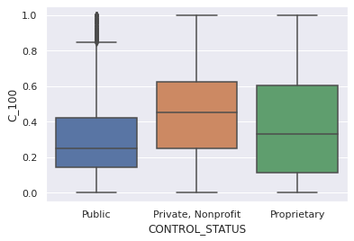
For completion rate by CONTROL

In [ ]:
rate_control = schools[['INSTNM', 'STATE', 'C_100', 'C_150', 'CONTROL_STATUS']]
rate_control
Out[ ]:
INSTNM STATE C_100 C_150 CONTROL_STATUS
0 Alabama A & M University Alabama 0.1052 0.2866 Public
1 University of Alabama at Birmingham Alabama 0.3816 0.6117 Public
2 Amridge University Alabama 0.2500 0.2500 Private, Nonprofit
3 University of Alabama in Huntsville Alabama 0.3109 0.5714 Public
4 Alabama State University Alabama 0.1462 0.3177 Public
6657 Pennsylvania State University-Penn State Wilke… Pennsylvania NaN NaN Public
6658 Pennsylvania State University-Penn State York Pennsylvania NaN NaN Public
6659 Pennsylvania State University-Penn State Great… Pennsylvania NaN NaN Public
6660 Pennsylvania State University-Penn State Harri… Pennsylvania NaN NaN Public
6661 Pennsylvania State University-Penn State Brand… Pennsylvania NaN NaN Public

6662 rows × 5 columns

In [ ]:
rate_control.groupby('CONTROL_STATUS')['C_100'].agg(['mean', 'count'])
Out[ ]:
mean count
CONTROL_STATUS
Private, Nonprofit 0.437661 1394
Proprietary 0.376065 2063
Public 0.318407 1730
In [ ]:
# set a grey background (use sns.set_theme() if seaborn version 0.11.0 or above) 
sns.set(style="darkgrid")

sns.boxplot(x= rate_control["CONTROL_STATUS"], y= rate_control["C_100"])
plt.show()

The boxplot shows that private instituitions has higher median completion rate than public instituition

In [ ]:
# set a grey background (use sns.set_theme() if seaborn version 0.11.0 or above) 
sns.set(style="darkgrid")

sns.boxplot(x= rate_control["CONTROL_STATUS"], y= rate_control["C_150"])
Out[ ]:
<AxesSubplot:xlabel='CONTROL_STATUS', ylabel='C_150'>

The addition school characteristics that I choose is the DEGREE TYPE. The rational behind this choise is that the higher the degree, the more challenging it becomes to complete

In [ ]:
rate_highdegree = schools[['INSTNM', 'STATE', 'C_100', 'C_150', 'HIGHDEG_TYPE']]
rate_icleveltype = schools[['INSTNM', 'STATE', 'C_100', 'C_150', 'ICLEVEL_TYPE']]
In [ ]:
# set a grey background (use sns.set_theme() if seaborn version 0.11.0 or above) 
sns.set(style="darkgrid")

sns.boxplot(x= rate_highdegree["HIGHDEG_TYPE"], y= rate_highdegree["C_100"])
plt.show()
In [ ]:
# set a grey background (use sns.set_theme() if seaborn version 0.11.0 or above) 
sns.set(style="darkgrid")

sns.boxplot(x= rate_icleveltype["ICLEVEL_TYPE"], y= rate_icleveltype["C_100"])
plt.show()
In [ ]:
# set a grey background (use sns.set_theme() if seaborn version 0.11.0 or above) 
sns.set(style="darkgrid")

sns.boxplot(x= rate_icleveltype["ICLEVEL_TYPE"], y= rate_icleveltype["C_150"])
plt.show()

Based on the boxplot above, less than 2 years degree has higher completion rates than 4 years degress


More To Explore