Exploring and describing data using Pandas

Share This Post

This notebook contains basic demonstration of how to explore and describe dataset with pandas. The basic outcomnes for this include:

  • importing python libraries
  • Load a data file into pandas
  • Examine the size and data types of a dataframe
  • Understand the relationship between DataFrame, Series and Index
  • Compute aggreate values from a pandas series
  • Compute grouped aggregrate values from a pandas dataframe
  • Order a data frame
  • Join two pandas dataframes for additional context
  • Provide numerical descriptions of a distribution
  • Visualize the distribution of a variable

Dataset

For this notebook, I used the MovieLens 25M Dataset. The Zip file is 250MB, and the files take about 1.2GB uncompressed. A quick documentation for the dataset is available here

Python modules

Most useful python functions are in modules. In other to use them, they need to be first imported

In [ ]:
import numpy as np
import pandas as pd
import matplotlib.pyplot as plt
import seaborn as sns

Reading CSV

In [ ]:
movies = pd.read_csv('../Data/ml-25m/movies.csv')
movies
Out[ ]:
movieId title genres
0 1 Toy Story (1995) Adventure|Animation|Children|Comedy|Fantasy
1 2 Jumanji (1995) Adventure|Children|Fantasy
2 3 Grumpier Old Men (1995) Comedy|Romance
3 4 Waiting to Exhale (1995) Comedy|Drama|Romance
4 5 Father of the Bride Part II (1995) Comedy
62418 209157 We (2018) Drama
62419 209159 Window of the Soul (2001) Documentary
62420 209163 Bad Poems (2018) Comedy|Drama
62421 209169 A Girl Thing (2001) (no genres listed)
62422 209171 Women of Devil’s Island (1962) Action|Adventure|Drama

62423 rows × 3 columns

The DataFrame

In [ ]:
movies.info()
<class 'pandas.core.frame.DataFrame'>
RangeIndex: 62423 entries, 0 to 62422
Data columns (total 3 columns):
 #   Column   Non-Null Count  Dtype 
---  ------   --------------  ----- 
 0   movieId  62423 non-null  int64 
 1   title    62423 non-null  object
 2   genres   62423 non-null  object
dtypes: int64(1), object(2)
memory usage: 1.4+ MB
  • RangeIndex: indexes 0 to n-1
  • 3 columns
    • 1 int64
    • 2 object – these store strings
  • 62423 rows
  • Kind of data
    • integer moviedID
    • string title
    • string genres
  • The data is about movies

-Each column is a series. It can be accessed like a disctionary

Series

  • An array with an index
  • All columns of the dataFrame share the same index
In [ ]:
movies['title']
Out[ ]:
0                          Toy Story (1995)
1                            Jumanji (1995)
2                   Grumpier Old Men (1995)
3                  Waiting to Exhale (1995)
4        Father of the Bride Part II (1995)
                        ...                
62418                             We (2018)
62419             Window of the Soul (2001)
62420                      Bad Poems (2018)
62421                   A Girl Thing (2001)
62422        Women of Devil's Island (1962)
Name: title, Length: 62423, dtype: object
In [ ]:
# How big is the series?
from turtle import title


print(movies['title'].size)
print(len(movies['title']))
print(movies['title'].shape)

#count count values not including missing values
movies['title'].count()
62423
62423
(62423,)
Out[ ]:
62423
  • .shape returns the array shape as a tuple — the array is one-dimensional with length 25M
  • .size returns the series size (length). len(…) is identical.
  • .count() counts values, not including missing value

Another DataFrame

Let’s load the ratings

In [ ]:
ratings = pd.read_csv('../Data/ml-25m/ratings.csv')
ratings.info()
<class 'pandas.core.frame.DataFrame'>
RangeIndex: 25000095 entries, 0 to 25000094
Data columns (total 4 columns):
 #   Column     Dtype  
---  ------     -----  
 0   userId     int64  
 1   movieId    int64  
 2   rating     float64
 3   timestamp  int64  
dtypes: float64(1), int64(3)
memory usage: 762.9 MB
  • Data has about 25M instances
  • Data contains
    • userId(int)
    • movieId(int)
    • rating(float)
    • timestamnp(int)
In [ ]:
ratings
Out[ ]:
userId movieId rating timestamp
0 1 296 5.0 1147880044
1 1 306 3.5 1147868817
2 1 307 5.0 1147868828
3 1 665 5.0 1147878820
4 1 899 3.5 1147868510
25000090 162541 50872 4.5 1240953372
25000091 162541 55768 2.5 1240951998
25000092 162541 56176 2.0 1240950697
25000093 162541 58559 4.0 1240953434
25000094 162541 63876 5.0 1240952515

25000095 rows × 4 columns

Aggregrate Functions

An aggregate function combines a series (or array) into a single value:

In [ ]:
ratings['rating'].mean()
Out[ ]:
3.533854451353085
In [ ]:
ratings['rating'].sum()
Out[ ]:
88346697.0

Alternate form – function from numpy

In [ ]:
np.sum(ratings['rating'])
Out[ ]:
88346697.0

Quantiles

Let’s see the quantile function

In [ ]:
ratings['rating'].quantile(0.25)
Out[ ]:
3.0
In [ ]:
ratings['rating'].quantile(0.75)
Out[ ]:
4.0

Interesting. 25% of the ratings is 4 or greater

Grouped Aggregrates

We can group by a column and compute aggreagrates within the group.
How many ratings per movie?

In [ ]:
ratings.groupby('movieId')['rating'].count()
Out[ ]:
movieId
1         57309
2         24228
3         11804
4          2523
5         11714
          ...  
209157        1
209159        1
209163        1
209169        1
209171        1
Name: rating, Length: 59047, dtype: int64

We can compute multiple aggregates at the same time:

In [ ]:
movie_stats = ratings.groupby('movieId')['rating'].agg(['mean', 'count'])
movie_stats
Out[ ]:
mean count
movieId
1 3.893708 57309
2 3.251527 24228
3 3.142028 11804
4 2.853547 2523
5 3.058434 11714
209157 1.500000 1
209159 3.000000 1
209163 4.500000 1
209169 3.000000 1
209171 3.000000 1

59047 rows × 2 columns

Finding Largest

We can get the 10 movies with the most ratings and 10 most rated movie

In [ ]:
movie_stats.nlargest(10, 'count')
Out[ ]:
mean count
movieId
356 4.048011 81491
318 4.413576 81482
296 4.188912 79672
593 4.151342 74127
2571 4.154099 72674
260 4.120189 68717
480 3.679175 64144
527 4.247579 60411
110 4.002273 59184
2959 4.228311 58773
In [ ]:
movie_stats.nlargest(10, 'mean')
Out[ ]:
mean count
movieId
27914 5.0 1
31945 5.0 1
83161 5.0 1
86975 5.0 1
92783 5.0 1
93991 5.0 1
95494 5.0 1
96799 5.0 1
99243 5.0 1
103875 5.0 1

Linking Data

Data can refer to other data

  • Ratings are instances themselves
  • But each connects a user to a movie

We can merge the two.

We want to combine our stats with movie info.

  • on=’movieId’ says to use the movieId column of the first frame instead of its index.
  • Matches values to index in other frame
In [ ]:
movie_info = movies.join(movie_stats, on='movieId')
movie_info
Out[ ]:
movieId title genres mean count
0 1 Toy Story (1995) Adventure|Animation|Children|Comedy|Fantasy 3.893708 57309.0
1 2 Jumanji (1995) Adventure|Children|Fantasy 3.251527 24228.0
2 3 Grumpier Old Men (1995) Comedy|Romance 3.142028 11804.0
3 4 Waiting to Exhale (1995) Comedy|Drama|Romance 2.853547 2523.0
4 5 Father of the Bride Part II (1995) Comedy 3.058434 11714.0
62418 209157 We (2018) Drama 1.500000 1.0
62419 209159 Window of the Soul (2001) Documentary 3.000000 1.0
62420 209163 Bad Poems (2018) Comedy|Drama 4.500000 1.0
62421 209169 A Girl Thing (2001) (no genres listed) 3.000000 1.0
62422 209171 Women of Devil’s Island (1962) Action|Adventure|Drama 3.000000 1.0

62423 rows × 5 columns

In [ ]:
movie_info.nlargest(10, 'count')
Out[ ]:
movieId title genres mean count
351 356 Forrest Gump (1994) Comedy|Drama|Romance|War 4.048011 81491.0
314 318 Shawshank Redemption, The (1994) Crime|Drama 4.413576 81482.0
292 296 Pulp Fiction (1994) Comedy|Crime|Drama|Thriller 4.188912 79672.0
585 593 Silence of the Lambs, The (1991) Crime|Horror|Thriller 4.151342 74127.0
2480 2571 Matrix, The (1999) Action|Sci-Fi|Thriller 4.154099 72674.0
257 260 Star Wars: Episode IV – A New Hope (1977) Action|Adventure|Sci-Fi 4.120189 68717.0
475 480 Jurassic Park (1993) Action|Adventure|Sci-Fi|Thriller 3.679175 64144.0
522 527 Schindler’s List (1993) Drama|War 4.247579 60411.0
108 110 Braveheart (1995) Action|Drama|War 4.002273 59184.0
2867 2959 Fight Club (1999) Action|Crime|Drama|Thriller 4.228311 58773.0

Average Movie Rating

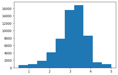
let’s look at the distribution of average movie rating:

In [ ]:
movie_info['mean'].describe()
Out[ ]:
count    59047.000000
mean         3.071374
std          0.739840
min          0.500000
25%          2.687500
50%          3.150000
75%          3.500000
max          5.000000
Name: mean, dtype: float64

Let’s make a histogram:

In [ ]:
plt.hist(movie_info['mean'])
plt.show()

And with more bins:

In [ ]:
plt.hist(movie_info['mean'], bins=50)
plt.show()

Wrapping Up

  • A dataframe consists of columns
  • Each column is a series: array with index
  • We can call info() method to quickly see
    • how many rows (instances)
    • what columns
    • data types
  • Aggregrates combine a series or array into a single value
    • Can compute over a whole series or over groups
  • Join combines frames
  • data description can be presented numerically and visually


More To Explore