Interferometric Synthetic Aperture Radar (InSAR) is based on the analysis of the phase difference between two images with different viewing geometry. You can read more about InSAR here. In this article, I will outline the steps for creating DEMS using strimapApp of ISCE. StripmapApp.py is an ISCE application, designed for interferometric processing of SAR data acquired with stripmap mode onboard platforms with precise orbits.  It implements InSAR processing flow for a pair of scenes from sensor raw data to geocoded, flattened interferograms. The workflow is highlighted below:

• Data Acquisition: The first step in any InSAR processing is data acquisition. For this tutorial, we will use ALOS Phased Array type L-band Synthetic Aperture Radar (ALOS PALSAR) data collected over Umnak Island in the Aleutians, Alaska. PALSAR is an L-band SAR data so this ensure that the InSAR coherence is high. However, the large temporal baseline is a limitation for InSAR application over an area where the feature changes rapidly in a short period.  We will use two acquisitions which cover Okmok Volcano right after its eruption in June 2008 (One in August 22 and the second in October 7). The raw data employed is available as staged data in strimapApp.
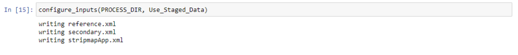
• Set-up input XML file for processing with StripmapApp: We require three input files for stripmap configuratins- reference.xml, secondary.xml and stripmap.xml. These files can be created with a text editor or by calling the ‘configure_inputs’ function of stripmapApp. This function takes two parameters- PROCESS_DIR which is the working directory and Use_Staged_Data which is a boolean value depending on wether we are using the staged data or not.

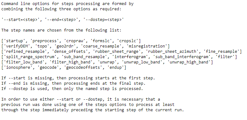
After downloading the data and setting the input xml files, we are ready to start processing with stripmapApp. We can see the full list of the processing steps using the command:

!stripmapApp.py –help –steps

• Data Preparation: The data preparation stage covers three processing steps- ‘startup’, ‘preprocess’ and ‘cropraw’.  preprocess step returned the neccesary files of each iimage pairs in separate folder while cropraw step would crop the raw data based on the region of interest if it was specified in the stripmapApp.xml
• SLC formation:  The step to generate SLC is ‘formslc’ as shown below.
  

  !stripmapApp.py stripmapApp.xml –start=formslc –end=formslc

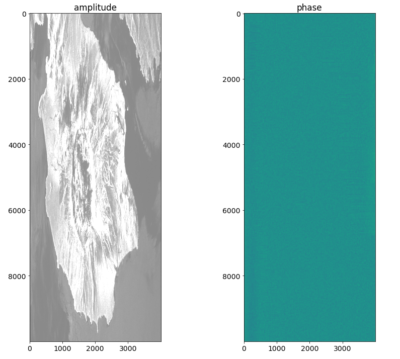
Single Look Complex Images contain both Amplitude and Phase information. The Amplitude and phase of one of the image pairs (August 22) is shown below:

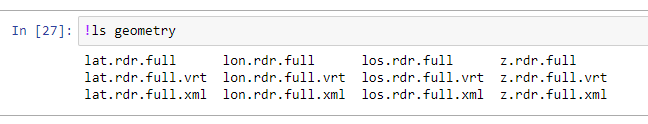
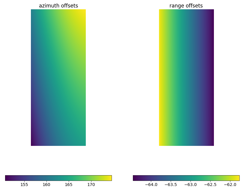
• Image co-registration: Image co-registration is done using a DEM. The steps in this stage include ‘verifyDEM’, ‘topo’, ‘geo2rdr’, ‘resampling’, ‘misregistration’, ‘refined_sample’ and other optional steps such as ‘dense_offsets’, ‘rubber_sheet’, ‘fine_resample’, ‘split_range_spectrum’ , ‘sub_band_resample’. ‘verifyDEM’ checks if the DEM was provided in the input xml file. If a DEM is not provided, then the app downloads SRTM DEM. The topo steps geolocate each pixels of the reference image using SAR acquisition geometry, platforms trajectory and existing DEM. The output of this step is saved in the ‘geometry’ directory. ‘geo2rdr’ step computes the range and azimuth time(radar coordinates) given the geo-coordinates of each pixels in the reference image (output of topo), acquisition geometry and orbit information of the secondary image. Azimuth.off: contains the offsets betwen reference and secondary images in azimuth direction. Range.off: contains the offsets betwen reference and secondary images in range direction

‘resampling’ resampled the secondary image to the same grid as the reference image, i.e., the secondary image is co-registered to the reference image. The output of this step is written to “coregisteredSlc” folder.

• Interferogram formation: At this step the reference image and refined_coreg.slc is used to generate the interferogram. This step also involves the removal of known patterns (flat earth).

!stripmapApp.py stripmapApp.xml –start=interferogram –end=interferogram

The results of the interferogram step is written to the “interferogram” folder:

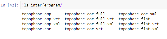
topophase.flat: flattened (geometrical phase removed) and multi-looked interferogram.(one band complex64 data).

topophase.cor: coherence and magnitude for the flattened multi-looked interferogram. (two bands float32 data).

topophase.cor.full: similar to topophase.cor but at full SAR resolution.

topophase.amp: amplitudes of reference amd secondary images. (two bands float32)

• Phase Filtering: A power spectral filter is applied to the multi-looked interferogram to reduce noise. The code for this is:

!stripmapApp.py stripmapApp.xml –start=filter –end=filter

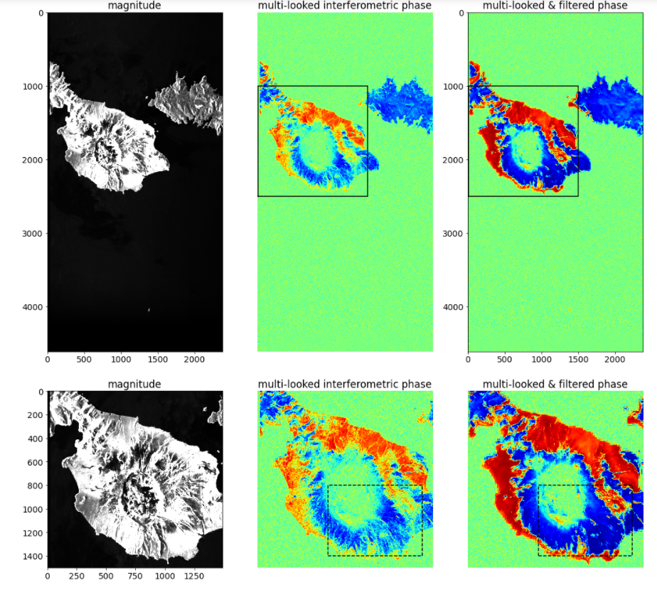
The visualization of the interferogram before and after filtering is shown below:

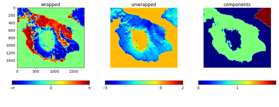
• Phase Unwrapping: At this step the wrapped phase of the filtered and multi-looked interferogram is unwrapped. The unwrapped interferogram is a two band data with magnitude and phase components.

!stripmapApp.py stripmapApp.xml –start=unwrap –end=unwrap

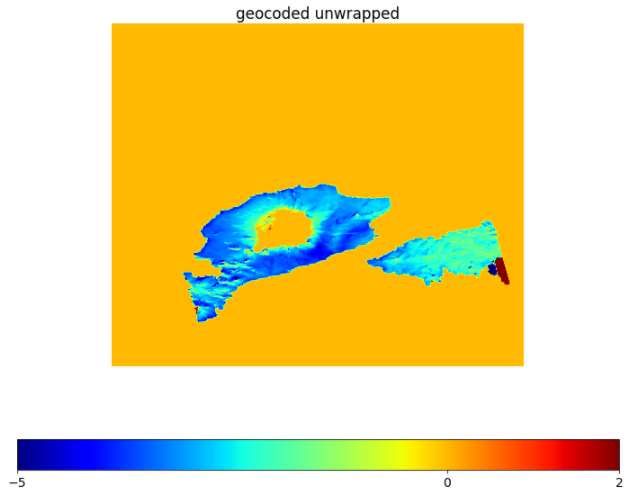
• Geocoding and Phase-to-height conversion

!stripmapApp.py stripmapApp.xml –start=geocode –end=geocode